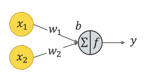
The neuron is just two matrices, one of intercepts, the other one of bias. if we have m inputs / features / independent variables $\mathbf{x}=[x_1,\cdots,x_m]^T$, we can write the neuron's function as a linear regression: $y=\mathbf{w}^T \mathbf{x}+b$, where intercepts are $\mathbf{w}=[w_1,\cdots,w_m]^T$.

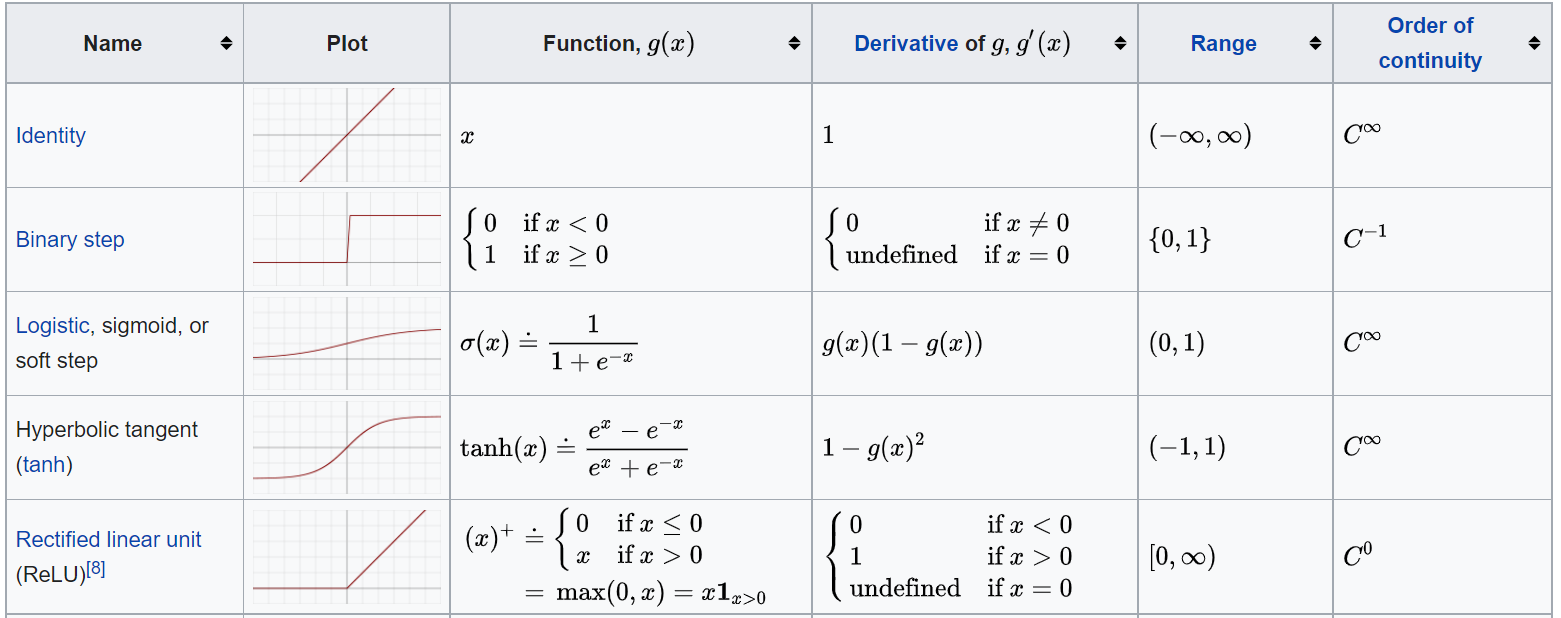
The neuron can also be for non-linear regression, through a non-linear function called the activation function. This function maps the $y$ into $y_{\text{hat}}$ within a certain range. Choice of the function is such that 1) the neuron can act like a switch: when y is below the threshold value, the neuron is turned off; otherwise it's turned on; 2) it is better to use a smooth function so that we can use its derivative for learning. The idea of gradient descent for learning is the same as what we discussed in the previous courses.
A typical activation function can be for example sigmoid function: $y =\cfrac{1}{1+exp(-x)}$. Some others are https://en.wikipedia.org/wiki/Activation_function:

import numpy as np
class Neuron:
def __init__(self,inputsize=3,weights=None,bias=None,activation='sigmoid'):
self.weights = weights
if not weights:
self.weights = np.random.normal(size=inputsize)
self.bias = bias
if not bias:
self.bias = np.random.rand()
if activation=='sigmoid':
self.activation = self.sigmoid
else:
self.activation = self.relu
def sigmoid(self,y):
return 1/(1+np.exp(-y))
def relu(self,y):
if y>0:
return y
return 0
def forward(self,x):
return self.activation(np.matmul(x,self.weights)+self.bias)
inputs = [1,2,3]
neuron = Neuron(activation='sigmoid')
print(neuron.forward(inputs))
neuron = Neuron(activation='relu')
print(neuron.forward(inputs))
0.8970168231830213 0
Now suppose we have two neurons in the first layer and one output neuron in the second layer. Each neuron is only connected to neurons in other layers, and each neuron is connected to ALL of the neurons in the adjacent layers.
We'd need clearer notations of the neurons. Let's denote the inputs with footnote $i$, the parameters in the first layer neurons with footnote $j$ (since we have two neurons in the first layer, j is either 1 or 2), and the parameters in the output neuron with footnote $l$ (since there's only one output neuron, $l=3$). The weights in each layer are denoted by both its start and end neurons, e.g., $w_{j=1,l=3}$ is the weight in neuron3 for input from neuron1.

For the output neuron3, since its input is the same as the output from the previous layer, we denote its input with $o_j,j \in \{1,2\}$.
For neurons 1 and 2 in the first layer: its input is denoted $o_i$, although, since we only have two layers, in our case $o_i=x_i$.
The activation function is denoted $\phi$. The target (ground truth) is $t$. The output from the output neuron3 is the estimate of the ground truth, denoted $\hat{y}$. Since we only have one output neuron, we also have $\hat{y}=o_l$.
For the intermediate result from the linear function, in neurons 1 and 2 for example, we use $\text{net}_j = (\sum_{i \in \{1,2,3\}} w_{ij} \cdot o_i) + b_j$. We'd also have for neuron1: $o_j = \phi(\text{net}_j)$.
For neuron3: $\text{net}_l= (\sum_{j \in \{1,2\}} w_{jl} \cdot o_j) + b_l$, and output $\hat{y}=o_l=\phi(\text{net}_l)$.
neuron1 = Neuron()
neuron2 = Neuron()
neuron3 = Neuron(inputsize=2)
o1 = neuron1.forward(inputs)
o2 = neuron2.forward(inputs)
y_hat = neuron3.forward([o1,o2])
print(o1,o2,y_hat)
0.9878072538614416 0.8883729264715795 0.35728001637405404
Suppose the target / ground truth / label is $t$. The loss function is mean squared error (as introduced in previous courses: measurement for regression problems): $e = \frac{1}{2} (t-\hat{y})^2$, where $\hat{y}=o_l$. Our goal is to approximate the target $t$ with our model, such that the output of the model is as close to the target as possible (i.e., minimize the mean squared error).
To do that, we need to be able to update our model parameters based on the error value. In linear regression, the parameters of the model would be the intercept and the bias. In a neural network, the parameters are all the weights and biases of all the neurons. Updating the parameters in a neural network is the same as in linear regression: through gradient descent. The only difference is the calculation of gradient: because neural networks are non-linear, we need to get the derivatives of a non-linear function.
We work it out backwards step-by-step.
derivative of the loss function
The derivative of the loss function (the mean squared error) is simply $\cfrac{\partial e}{\partial o_l} = o_l - t$.
To update the last neuron's weights and bias, we'd need the derivative of the error $e$ with respect to each weight and bias.
To do that, we first get the derivative of the activation function (suppose it's a sigmoid) with respect to $\text{net}_l$, then the derivative of the linear function with respect to the weights and bias.
derivative of the activation function
Neuron3's sigmoid function's derivative with respect to its input $\text{net}_l$ is:
$\cfrac{\partial o_l}{\partial \text{net}_l} = \cfrac{\partial \phi(\text{net}_l)}{\partial \text{net}_l} = o_l \cdot (1-o_l)$
A step-by-step calculation is here: https://towardsdatascience.com/derivative-of-the-sigmoid-function-536880cf918e
derivative of the linear function
The derivative of $\text{net}_l$ with respect to each of neuron3's intercept $w_{jl}$ is:
$\cfrac{\partial \text{net}_l}{\partial w_{jl}} = \cfrac{\partial [(\sum_{j \in \{1,2\}} w_{jl} o_j) + b_l]}{\partial w_{jl}}=o_j$
putting it all together with chain rule:
According to the chain rule, the complete derivative from loss to intercept $w_{jl}$ in the last neuron (neuron3) is:
$\Delta_{w_{jl}}=\cfrac{\partial e}{\partial w_{jl}}=\cfrac{\partial e}{\partial o_l} \cdot \cfrac{\partial o_l}{\partial \text{net}_l} \cdot \cfrac{\partial \text{net}_l}{\partial w_{jl}} = (o_l - t) \cdot (o_l \cdot (1-o_l)) \cdot o_j$.
For bias, $\Delta_{b_l}=(o_l - t) \cdot (o_l \cdot (1-o_l))$.
the gradient descent and updating model parameters:
According to the gradient descent algorithm, we'd update the original weight and bias values of the neuron3 with:
$w_{jl} \gets w_{jl} - \eta \Delta_{w_{jl}}$ and $b_{l} \gets b_{l} - \eta \Delta_{b_{l}}$
In order to understand the wikipedia page: https://en.wikipedia.org/wiki/Backpropagation, we change our notations slightly:
We use $\delta_l = (o_l - t) \cdot (o_l \cdot (1-o_l))$ and rewrite the above to:
$w_{jl} \gets w_{jl} - \eta \delta_l o_j$ and $b_{l} \gets b_{l} - \eta \delta_l$.
This formula will be universal for all neurons.
A quick recap of gradient descent: the gradient of the loss function points out the direction of the update: if gradient is negative, the weight needs to increase; if the gradient is positive, the weight needs to decrease. The learning rate $\eta$ controls the size of the update: if the step is too big, we risk oscillating and never converging. If the step is too small, it may take too long to reach the minimum. https://en.wikipedia.org/wiki/Gradient_descent

extend it to any neurons (not just the output neuron):
For any neurons that are not the output neuron, it would need a longer chain of derivatives backwards. For neuron1 for example:
$o_{j=1}=\phi(\text{net}_j) = \phi(\sum_{i} (w_{ij} \cdot o_i) + b_j)$
The chain rule from error $e$ to $w_{ij}$ is:
$\cfrac{\partial e}{\partial w_{ij}}=\cfrac{\partial e}{\partial o_l} \cdot \cfrac{\partial o_l}{\partial \text{net}_l} \cdot \cfrac{\partial \text{net}_l}{\partial o_j} \cdot \cfrac{\partial o_j}{\partial \text{net}_j} \cdot \cfrac{\partial \text{net}_j}{\partial w_{ij}}=(o_l - t) \cdot (o_l \cdot (1-o_l)) \cdot w_{jl} \cdot (o_j \cdot (1-o_j)) \cdot o_i$
Again we use $\delta_j=\delta_l \cdot w_{jl} \cdot (o_j \cdot (1-o_j))$ and rewrite:
$w_{ij} \gets w_{ij} - \eta \delta_j o_i$.
In fact, if there would be multiple output neurons, we need to add the gradients together (as on the wikipedia page):
$\delta_j=(\sum_l \delta_l \cdot w_{jl}) \cdot (o_j \cdot (1-o_j))$
But the update rule stays the same for all neurons: $w_{ij} \gets w_{ij} - \eta \delta_j o_i$.
This backward pass, as opposed to the forward pass before, is called backpropagation.
Now we rewrite the Neuron class to include the backward pass.
class Neuron:
def __init__(self,inputsize=3,weights=None,bias=None,activation='sigmoid'):
self.weights = weights
if not weights:
self.weights = np.random.normal(size=inputsize)
self.bias = bias
if not bias:
self.bias = np.random.rand()
if activation=='sigmoid':
self.activation = self.sigmoid
else:
self.activation = self.relu
def sigmoid(self,y):
return 1/(1+np.exp(-y))
def relu(self,y):
if y>0:
return y
return 0
def forward(self,x):
self.o_i = x
self.o_j = self.activation(np.matmul(x,self.weights)+self.bias)
return self.o_j
def backward(self,t=None,y_hat=None,delta_l=None,w_l=None,
learning_rate=0.1,output_neuron=False):
''' if output_neuron is True, the neuron is the output neuron.
Otherwise it's a neuron in an internal layer. '''
if output_neuron:
delta_j = (y_hat - t) * self.o_j * (1 - self.o_j)
else:
delta_j = np.matmul(delta_l,w_l)
self.delta_j = delta_j
new_weights = []
for i,w in enumerate(self.weights):
new_weights.append(w - learning_rate * delta_j * self.o_i[i])
self.weights = new_weights
self.bias = self.bias - learning_rate * delta_j
Set up the network:
t = 1.0
inputs = [1,2,3]
neuron3 = Neuron(inputsize=2)
neurons = []
for j in range(2):
neurons.append(Neuron(activation='sigmoid'))
for j in range(2):
print('neuron {}: {}.'.format(j,neurons[j].weights))
print('output neuron: {}.'.format(neuron3.weights))
neuron 0: [-0.41451339 -1.77081177 -1.15804613]. neuron 1: [-1.78363994 -1.89654933 -0.46369448]. output neuron: [-0.43875046 0.81212614].
Run forward pass and backward pass once:
o_j = []
for j in range(2):
o_j.append(neurons[j].forward(inputs))
y_hat = neuron3.forward(o_j)
neuron3.backward(t=t,y_hat=y_hat,output_neuron=True)
delta_l = neuron3.delta_j
for j in range(2):
w_l = neuron3.weights[j]
neurons[j].backward(delta_l=[delta_l],w_l=[w_l],output_neuron=False)
for j in range(2):
print('neuron {}: {}.'.format(j,neurons[j].weights))
print('output neuron: {}.'.format(neuron3.weights))
print('estimate: {}, error: {}.'.format(y_hat,t-y_hat))
neuron 0: [-0.41853992193557854, -1.778864844034011, -1.1701257432807464]. neuron 1: [-1.7761864539890273, -1.8816423677625997, -0.4413340381348142]. output neuron: [-0.4387411310235029, 0.8121493546532328]. estimate: 0.6131035670318141, error: 0.3868964329681859.
# your training code below
inputs = [[1,2,3],[4,5,6]]
t = [1.0,0.7]
# your training code below
# your new class definition and training code below
t = [[1.0,0.0,0.0],[0.0,1.0,0.0]]
# your new class definition and training code below
# your new class definition below