recurrent neural network¶

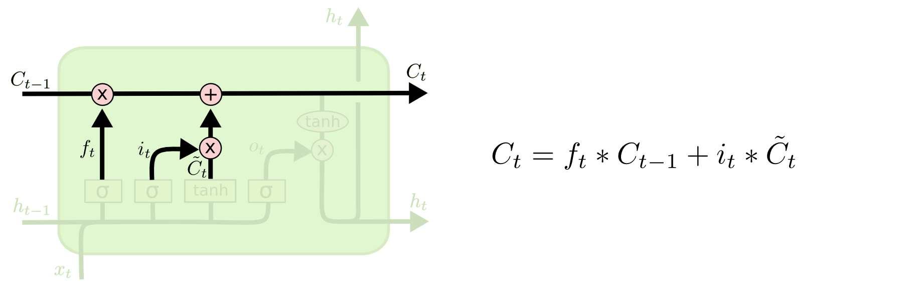
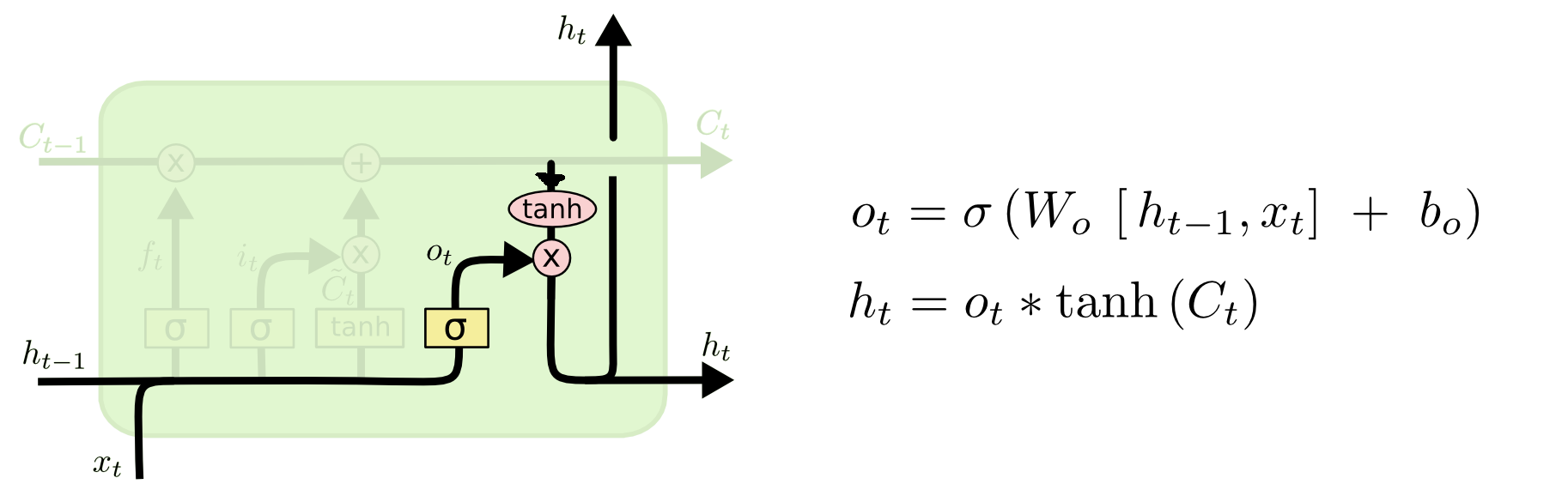
This notebook's LSTM part is a shortened (and simplified) version of colah's blog.

1. why recurrent neural network, and what is it¶

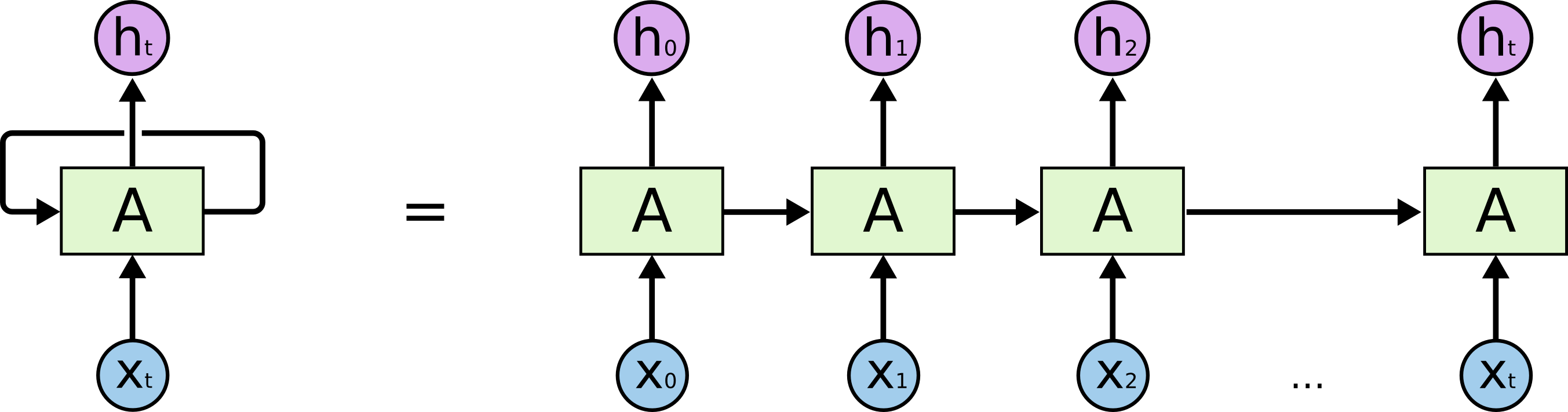
Because processing of sequence data is incremental: the understanding of the current information is always based on information in the past. Like natural language, or timeseries: our understanding of the new word / new data point is based on information gained from previous words or data. The process of cumulating information from each record is recurrent: one processing center (e.g., our brain) uses its own output from the previous cycle as input to the current cycle. Graphically it's commonly depicted with a loop:

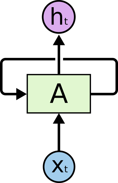
$x$ is the input sequence, $h$ is the output sequence, or understanding of the input sequence. $t$ denotes the position of the element in the sequence, or we can also say the element we receive at the current time $t$. $A$ is the processing center, i.e., the model or our brain.

Another common way to depict the temporal dimension of recurrent processing is to unroll it along the timeline:

2. long short term memory (LSTM)¶

It is a classic recurrent neural network. It solves the problem of the neural network forgetting old but important information. LSTM remembers relevant past information through gates. One LSTM cell looks like this:

We break it down by its gates:

a). the direct path throughout time:

The memory cell output from previous time step goes into the current memory cell, with an updated memory (the update is decribed later).

b). the first gate: the forget gate

The calculation of $f_t$ should be familiar to you: it's the same format as in our previous class. The $\sigma$ is the sigmoid function. The rest is a linear function with intercept $W$ and bias $b$. The input is a bit different: it's not the actual input $x$, but a mixture of preivous output $h_{t-1}$ and current input $x_t$.

How can we understand it as a gate?

The linear function extracts some kind of features from not only the current input, but also the previous understanding of the past sequence. Then the sigmoid function serves as a switch that opens or closes the gate. $f_t$ is the forget weight: if the output of sigmoid is close to 0, it means to forget more of the previous memory; if the sigmoid output is close to 1, it means to "keep remembering". The forget weight is multiplied with previous memory $C_{t-1}$. That's the yellow circle with a multiplicator.

c). the second gate: the input gate

The input gate $i_t$ is again in a very familiar format. The sigmoid opens or closes the gate. This gate weighs the importance of a memory update (a.k.a. cell update) denoted $\tilde{C}_t$.

The cell update calculation is again familiar, only with a different activation function: the hyperbolic tangent. Remember from the previous class, how the tanh activation function has a different output range and derivatives.

This newly acquired memory triggered by the new input is weighed by the input gate and then added to the old memory $C_{t-1}$ to form the new memory cell state $C_t$. That's the yellow circle with a plus:

d). the third gate: the output gate

By now you should be able to recognize the $o_t$ as a gate. It again serves as a weight factor or a "switch", this time to weigh the importance of the new memory $C_t$ to our understanding ($h_t$) of the input sequence.

Every LSTM cell therefore has two outputs: the memory cell state, and the actual output. The two outputs will become inputs to the LSTM cell in the next time step. This is important to remember when we use the off-the-shelf LSTM cells from pytorch in the next class, otherwise you'd be wondering why there are two outputs and we only use one.

3. the autoencoder structure¶

Autoencoders are not necessarily recurrent neural networks, it's just a very common structure consisting of an encoder and a decoder. The encoder and decoder can be any sort of neural networks, depending on the task. They can of course be LSTMs, f_tor sequential data.

This image is from here.

Autoencoders are a type of generative, unsupervised learning algorithm. Originally, an autoencoder is designed to 1. learn the hidden features of the high dimensional inputs through the encoder (output from the encoder, the green block in the middle of the figure above, is a feature map), and 2. the decoder tries to reconstruct the original input from the feature map. If the final output from the decoder ($\hat{X}$) is very similar to the original input to the encoder ($X$), we can say that the feature map is an accurate representation. It can therefore also be seen as a regularization tool, and the feature map can be used for further processing, for example as input to a classification model, etc.

But of course the autoencoder can be more than that. We can build on the generative nature of the decoder to do other things such as translation, or generation of image captions (image to text). In this case, the decoder is no longer trying to reconstruct the original input, but trying to generate new output based on the feature map -- e.g., English in, French out, or image in, text out. The structure would then change to:

The autoencoder structure is very often used in NLP-related algorithms, for example in transformer.

We are going to build a simple LSTM-autoencoder using pytorch's built-in LSTM layer in our next class.

4. the attentional network¶

Another concept you need to know before we get to the NLP algorithms such as transformer, is attention. This is just a huge weight matrix that fully connects two sets of data, with the purpose of showing where the two sets of data have the strongest correlation.

There's an interesting visualization of attention between words in a sentence here:

In an autoencoder, the attentional network usually sits right between the encoder and the decoder, connecting the extracted features of the encoder and the decoder. This weight matrix indicates which part of the input $X$ is more important to the current $Y_t$.

Now the autoencoder structure is changed to:

The attention calculation can be either additive or multiplicative. The additive attention is the earlier version and the original attention idea. The multiplicative attention is later developed to enhance computational performance, and is therefore more commonly used in the newer NLP models such as transformer.

If you have time, here is an explanation of the difference and implementation in pytorch. Specifically for the multi-head multiplicative attention mechanism used in transformers, here is a step-by-step explanation.